Cortical Recording During Behavior

Electrophysiology

Methods

Analysis pipeline for cortical LFP recordings across behavioral contexts.

Author

Mursel Karadas

Published

November 1, 2024

%load_ext autoreload
%autoreload 2

import logging
# Set logging to only show warnings and errors
logging.getLogger().setLevel(logging.WARNING)
import warnings

# Suppress specific warnings (e.g., RuntimeWarnings)
warnings.filterwarnings('ignore', category=RuntimeWarning)

%matplotlib inline

import brian2.only as b2
from brian2 import np
import matplotlib.pyplot as plt
import cleo
import cleo.utilities
# the default cython compilation target isn't worth it for
# this trivial example
b2.prefs.codegen.target = "numpy"
seed = 18810929
b2.seed(seed)
np.random.seed(seed)
cleo.utilities.set_seed(seed)

cleo.utilities.style_plots_for_docs()

# colors
c = {
    "light": "#df87e1",
    "main": "#C500CC",
    "dark": "#8000B4",
    "exc": "#d6755e",
    "inh": "#056eee",
    "accent": "#36827F",
}

N = 1000
n_e = int(N * 0.8)
n_i = int(N * 0.2)
n_ext = 500

neurons = b2.NeuronGroup(
    N,
    "dv/dt = -v / (10*ms) : 1",
    threshold="v > 1",
    reset="v = 0",
    refractory=2 * b2.ms,
)
ext_input = b2.PoissonGroup(n_ext, 24 * b2.Hz, name="ext_input")
cleo.coords.assign_coords_rand_rect_prism(
    neurons, xlim=(-0.2, 0.2), ylim=(-0.2, 0.2), zlim=(0.55, 0.9)
)
# need to create subgroups after assigning coordinates
exc = neurons[:n_e]
inh = neurons[n_e:]

w0 = 0.06
syn_exc = b2.Synapses(
    exc,
    neurons,
    f"w = {w0} : 1",
    on_pre="v_post += w",
    name="syn_exc",
    delay=1.5 * b2.ms,
)
syn_exc.connect(p=0.1)
syn_inh = b2.Synapses(
    inh,
    neurons,
    f"w = -4*{w0} : 1",
    on_pre="v_post += w",
    name="syn_inh",
    delay=1.5 * b2.ms,
)
syn_inh.connect(p=0.1)
syn_ext = b2.Synapses(
    ext_input, neurons, "w = .05 : 1", on_pre="v_post += w", name="syn_ext"
)
syn_ext.connect(p=0.1)

# we'll monitor all spikes to compare with what we get on the electrode
spike_mon = b2.SpikeMonitor(neurons)

net = b2.Network([neurons, exc, inh, syn_exc, syn_inh, ext_input, syn_ext, spike_mon])
sim = cleo.CLSimulator(net)
cleo.viz.plot(exc, inh, colors=[c["exc"], c["inh"]], scatterargs={"alpha": 0.6});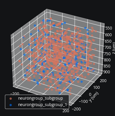

from cleo import ephys
from mpl_toolkits.mplot3d import Axes3D

array_length = 0.4 * b2.mm  # length of the array itself, not the shank
tetr_coords = ephys.tetrode_shank_coords(array_length, tetrode_count=3)
poly2_coords = ephys.poly2_shank_coords(
    array_length, channel_count=32, intercol_space=50 * b2.um
)
poly3_coords = ephys.poly3_shank_coords(
    array_length, channel_count=32, intercol_space=30 * b2.um
)
# by default start_location (location of first contact) is at (0, 0, 0)
single_shank = ephys.linear_shank_coords(
    array_length, channel_count=8, start_location=(-0.2, 0, 0) * b2.mm
)
# tile vector determines length and direction of tiling (repeating)
multishank = ephys.tile_coords(
    single_shank, num_tiles=3, tile_vector=(0.4, 0, 0) * b2.mm
)

fig = plt.figure(figsize=(8, 8))
fig.suptitle("Example array configurations")
for i, (coords, title) in enumerate(
    [
        (tetr_coords, "3-tetrode shank"),
        (poly2_coords, "32-channel Poly2 shank"),
        (poly3_coords, "32-channel Poly3 shank"),
        (multishank, "Multi-shank"),
    ],
    start=1,
):
    ax = fig.add_subplot(2, 2, i, projection="3d")
    x, y, z = coords.T / b2.um
    ax.scatter(x, y, z, marker="x", c="black")
    ax.set(
        title=title,
        xlabel="x [μm]",
        ylabel="y [μm]",
        zlabel="z [μm]",
        xlim=(-200, 200),
        ylim=(-200, 200),
        zlim=(400, 0),
    )
plt.show()

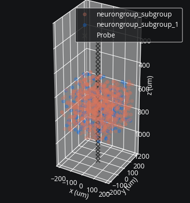
coords = ephys.linear_shank_coords(1 * b2.mm, 32, start_location=(0, 0, 0.2) * b2.mm)
probe = ephys.Probe(coords, save_history=True)
cleo.viz.plot(
    exc,
    inh,
    colors=[c["exc"], c["inh"]],
    zlim=(0, 1200),
    devices=[probe],
    scatterargs={"alpha": 0.3},
);

mua = ephys.MultiUnitActivity()
ss = ephys.SortedSpiking()

tklfp = ephys.TKLFPSignal()
rwslfp = ephys.RWSLFPSignalFromSpikes()

probe.add_signals(mua, ss, tklfp, rwslfp)

sim.set_io_processor(cleo.ioproc.RecordOnlyProcessor(sample_period=1 * b2.ms))
sim.inject(
    probe,
    exc,
    tklfp_type="exc",
    ampa_syns=[syn_exc[f"j < {n_e}"], syn_ext[f"j < {n_e}"]],
    gaba_syns=[syn_inh[f"j < {n_e}"]],
)
sim.inject(probe, inh, tklfp_type="inh")

CLSimulator(io_processor=RecordOnlyProcessor(sample_period=1. * msecond, sampling='fixed', processing='parallel'), devices={Probe(name='Probe', save_history=True, signals=[MultiUnitActivity(name='MultiUnitActivity', probe=..., r_noise_floor=80. * umetre, threshold_sigma=4, spike_amplitude_cv=0.05, r0=5. * umetre, recording_recall_cutoff=0.001, eap_decay_fn=<function Spiking.<lambda> at 0x17756cae0>, simulate_false_positives=True, collision_prob_fn=<function MultiUnitActivity.<lambda> at 0x177612980>), SortedSpiking(name='SortedSpiking', probe=..., r_noise_floor=80. * umetre, threshold_sigma=4, spike_amplitude_cv=0.05, r0=5. * umetre, recording_recall_cutoff=0.001, eap_decay_fn=<function Spiking.<lambda> at 0x17756cae0>, simulate_false_positives=True, snr_cutoff=6, collision_prob_fn=<function SortedSpiking.<lambda> at 0x177612de0>), TKLFPSignal(name='TKLFPSignal', probe=..., uLFP_threshold=1. * nvolt, _lfp_unit=uvolt), RWSLFPSignalFromSpikes(name='RWSLFPSignalFromSpikes', probe=..., amp_func=<function mazzoni15_nrn at 0x17750d120>, pop_aggregate=False, wslfp_kwargs={}, _lfp_unit=1, tau1_ampa=2. * msecond, tau2_ampa=0.4 * msecond, tau1_gaba=5. * msecond, tau2_gaba=250. * usecond, syn_delay=1. * msecond, I_threshold=0.001, weight='w')])})

sim.run(250 * b2.ms)

INFO       No numerical integration method specified for group 'neurongroup', using method 'exact' (took 0.01s). [brian2.stateupdaters.base.method_choice]

fig, axs = plt.subplots(3, 1, sharex=True, layout="constrained", figsize=(6, 6))

spikes_are_exc = spike_mon.i < n_e
# need to map sorted unit index to cell type
i_sorted_is_exc = np.array([ng == exc for (ng, i) in ss.i_ng_by_i_sorted])
sorted_spikes_are_exc = i_sorted_is_exc[ss.i]

for celltype, i_all, i_srt in [
    ("exc", spikes_are_exc, sorted_spikes_are_exc),
    ("inh", ~spikes_are_exc, ~sorted_spikes_are_exc),
]:
    axs[0].plot(
        spike_mon.t[i_all] / b2.ms,
        spike_mon.i[i_all],
        ".",
        c=c[celltype],
        rasterized=True,
        label=celltype,
        ms=2,
    )
    axs[1].plot(
        ss.t[i_srt] / b2.ms,
        ss.i[i_srt],
        ".",
        c=c[celltype],
        label=celltype,
        rasterized=True,
    )
axs[0].legend()
axs[0].set(ylabel="NeuronGroup index", title="ground-truth spikes")
axs[1].set(title="sorted spikes", ylabel="sorted unit index")

axs[2].plot(mua.t / b2.ms, mua.i, "w.", rasterized=True)
axs[2].set(
    title="multi-unit activity",
    ylabel="channel index",
    xlabel="time (ms)",
    ylim=[-0.5, probe.n - 0.5],
);
plt.show()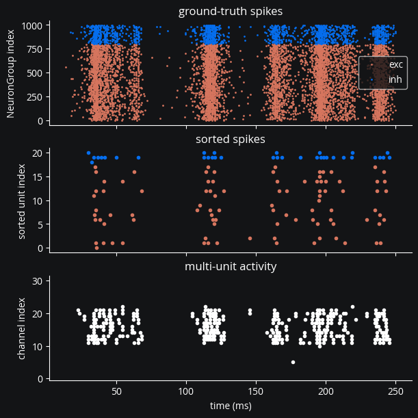

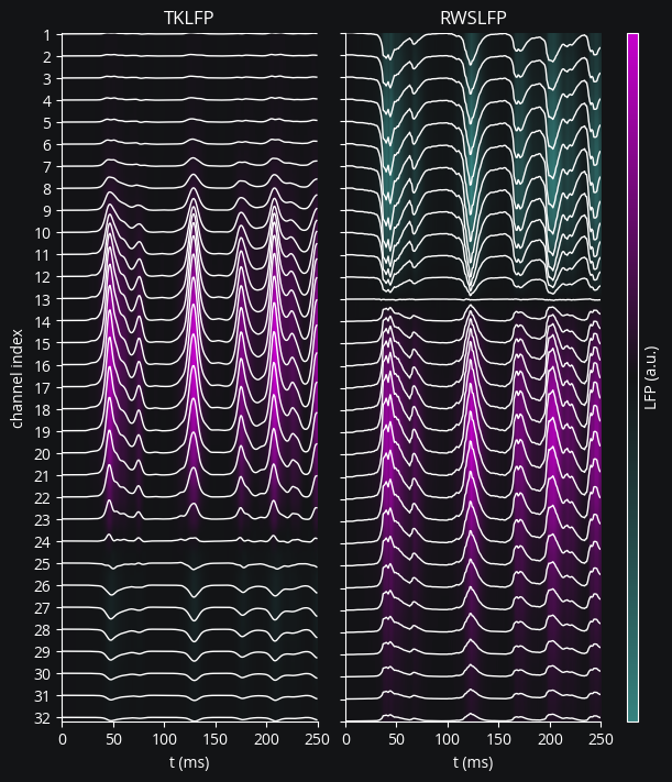
from matplotlib.colors import LinearSegmentedColormap

fig, axs = plt.subplots(1, 2, figsize=(6, 7), sharey=False, layout="constrained")
for ax, lfp, title in [
    (axs[0], tklfp.lfp / b2.uvolt, "TKLFP"),
    (axs[1], rwslfp.lfp, "RWSLFP"),
]:
    channel_offsets = -np.abs(np.quantile(lfp, 0.9)) * np.arange(probe.n)
    lfp2plot = lfp + channel_offsets
    ax.plot(lfp2plot, color="white", lw=1)
    ax.set(
        yticks=channel_offsets,
        xlabel="t (ms)",
        title=title,
    )

    extent = (0, 250, lfp2plot.min(), lfp2plot.max())
    cmap = LinearSegmentedColormap.from_list("lfp", [c["accent"], "#131416", c["main"]])
    im = ax.imshow(
        lfp.T,
        aspect="auto",
        cmap=cmap,
        extent=extent,
        vmin=-np.max(np.abs(lfp)),
        vmax=np.max(np.abs(lfp)),
    )

fig.colorbar(im, aspect=60, label="LFP (a.u.)", ticks=[])

axs[0].set(
    ylabel="channel index",
    yticklabels=range(1, 33),
)
axs[1].set(yticklabels=[]);
plt.show()